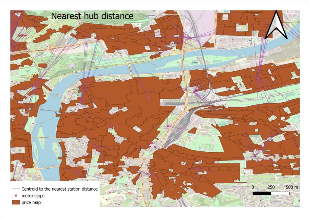
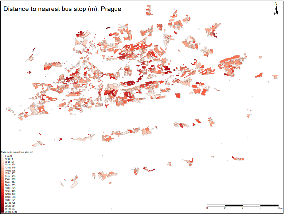
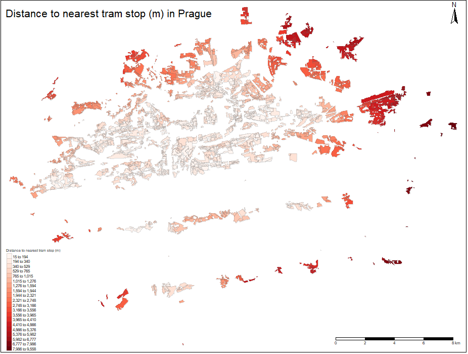
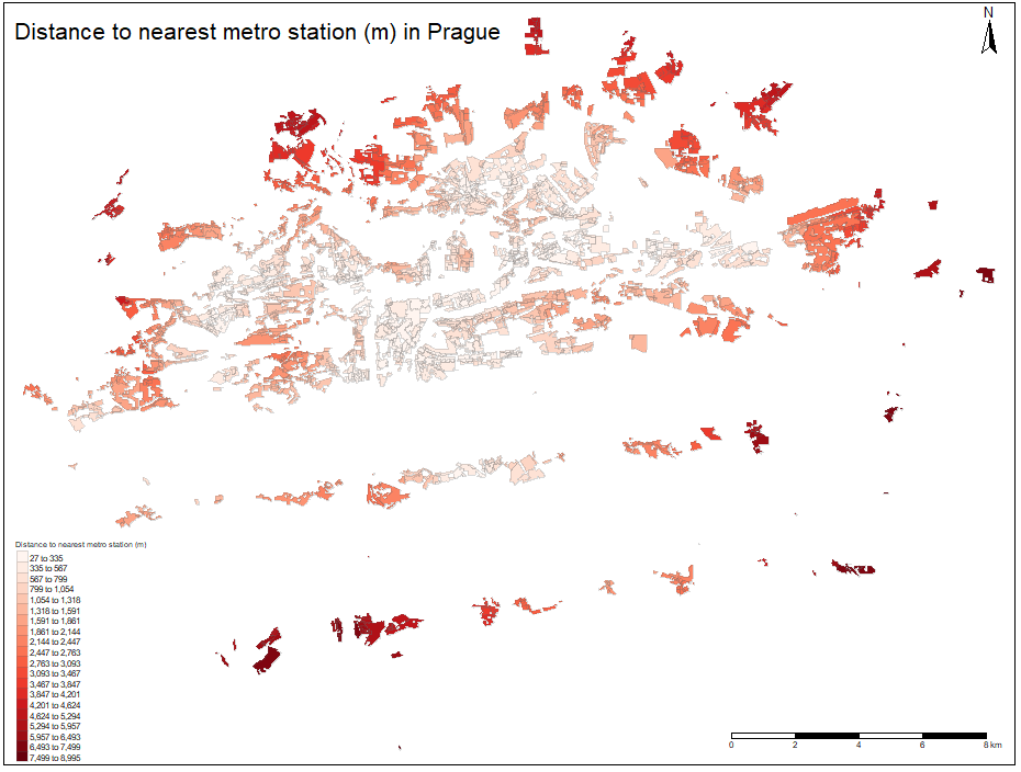
Using distance to nearest hub function in QGIS, for each public transport stop layer, the nearest hub distance to the centroid of each polygon is obtained. The snapshot from the nearest metro station distance output is plotted on the figure on the next page. The same procedure is applied to Tram,Train and Bus stops and by using spatial join, each hub distance is assigned to corresponding polygon. After converting the area of the polygons to square meters, all variables from the model scheme are obtained and the project will proceed with empirical data analysis.

As the land area can be observed directly from any other plot, the figure is not included. By visual observation it seems that the largest polygons are located on the city outskirts rather than in the city center. This corresponds with the urban design as the city center contains mostly historical apartment blocks whereas on the outskirts large concrete panel housing estates, especially on the eastern (Černý Most) and southern (Jižní Město) tips were build in the past 60 years ¹.

Starting with the analysis of price, figure below depicts the spatial distribution of residential land prices in Prague. One can see that the most valuable land is clustered arround historical city center whereas the least prices per square meter can be found on the outskirts of the cities. By observing the map, it seems that there is significant cluster of lower value land in the northern part of the city, in the Bohnice Municipality. It might correspond with the fact that this part of the city does not have any tram or metro stop nearby and it is available only by bus. This assumption will be further tested.

To investigate all values, summary statistics table of the dataset is printed below. Minimal value of price seems to be outlier as it is more than 20 times smaller than 25% quantile. The mean price is approximately 17% larger than median, indicating strong influence of large value observations. Regarding the area, the observation with minimal value has the same properties as the price as it is same polygon. The increase is much steeper, as the mean area is 2.31 times larger than the median. When investigating the distances, the smallest value with almost 5 meters is the minimal value of the nearest bus distance. Such small value does not seem to be realistic, however it is a payoff for the way how the distances were calculated. For the maximal values of distances, it can be observed that some areas are disconnected to the rail modes as the highest distance for metro, train and tram are not in walk-able radius. Overall, the variables will be further analysed in following sections, taking spatial properties into consideration.

Sumarry statistics of the dataset

To obtain residential land only from the Price map it is necessary to find out which polygons corresponds to residential usage.
Area Usage Plan spatial dataset from Institute of Planning and Development is used ¹ to label residential polygons. This dataset contains vector polygons with encoded type of usage of the areas. For the analysis, following types of areas was used – pure residential, general residential, general mixed, city core mix. The snapshot from filtered output is plotted on the figure.

To obtain price map polygons for residential areas only, Extract By Location process in QGIS, with geometric predicate „contains“ is used as shown on the figure.

The final output is the Price map of residential areas. Each polygon represents residential or mixed area with price per square meter attribute. It represents approximately 35\% of all polygons, comparison between the original price map dataset and residential price map is depicted on the figure below.

The main data source for the analysis is Price Map obtained as an open data source from Prague Institute of Planning and Development ¹. The Price Map is spatial database that contains vector polygons with price attribute. The price attribute is understood as price of land per square meter. However since it does not specify whether the land use is residential, commercial or other, it will have to be further processed to filter out non residential areas. All data that will be used in the analysis are listed below.

•  Price map shapefile
•  Area Usage Plan shapefile
•  Prague Integrated Transport System stops shapefile
•  Prague Integrated Transport System stops extra descriptions csv
•  City of Prague borders shapefile