As mentioned above in the report, our final model is gamma distributed model stated above.
The diagnostics plot of final model are depicted on figure below:

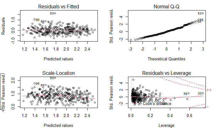
Compared with diagnostic plot of classical general linear model, we observe differences. The outlying observations are different, however none of these outliers lies in the Cook´s distance region. In the Residual vs Fitted plot we got rid of the pattern when the observations were clustered in lines, now they seems to be more scattered.
On the Normal Q-Q plot, we can see outlying observation number 53. We might have slightly improve the model fit by removing this point however as we are not sure if it caused by measuring error, we have decided to leave it there.
On the Scale location plot we can observe that the red line is more horizontal which indicates better fit of the model compared with the final model in question 1.
On the residual vs Leverage plot the large cluster on the left is still visible. However more observations seems to be scattered which also indicates better fit.

From visual inspection of the spatial distribution for nearest tram stop distance, it seems that the majority of the residential land areas is well connected to the tram network as these polygons tends to have short distance and they are neighboured by polygons with same characteristics in terms of tram network’s connectivity. Polygons with higher values of Moran statistics tends to be arranged in the north and east outskirts of the city. It can be seen from the figure that tram lines are missing in these neighbourhoods and their inhabitants have to rely on buses and individual forms of transportation. As mentioned before, these areas had been connected during the city expansion in 1922 or later, however it seems that no progress of expanding the tram network north east from center has been achieved since then. The situation will most likely remain same as no solution has been proposed yet and these areas aren’t included in the Official Development brochure for the next decade ¹.

When comparing spatial distribution of local moran statistics for metro with the same statistical model for bus, different spatial variation of Moran’s values can be observed. From all statistically significant polygons, the most frequent areas are light blue, corresponding to low values areas neighbouring with those with high value of Moran statistics. As all light blue areas are aligned near metro lines, this pattern confirms empirical observations. Besides one red polygon west of the city center, any other disconnected area lies on the outskirts of the city, where metro network doesn’t reach these neighbourhood. As the city will most likely expand, this can be early indicator of necessity to build ring line in the underground transportation system.

Spatial distribution of moran statistics for nearest bus stop distance is depicted. Note: The bus lines and stops are not plotted unlike for other modes. As the bus network and its stops are very densed, whole figure would become disorganized. We can observe that majority of statistical significant polygons are low values neighbouring with another low values. The implication from the model can be that these locations are well connected to the bus network. On the eastern end of the city we can observe a large red polygon. It is located in the Horní Počernice municipality, which is one of the most recent that was connected to Prague in 1974. The municipality has suburban character and this polygon is actually surrounding very frequently used train station so the usage of buses or trams was not prioritized during the development. From the figure it can be inspected that many regions are well connected to the bus network, however they are neighboured by areas with higher distances to nearest bus station. It seems that this pattern copies the historical development as these areas are located near the original border before the city expansion in 1922 ¹.

When investigating local clustering patterns of land area in square meters, large red polygons can be observed on the outskirt of the city. These neighbourhoods have suburban character consisting of detached houses with large gardens. Such characteristic is typical for larger areas that are neighbouring with another large areas. When interpreting small polygons in the city center, the only explanation with respect to area can be that these polygons consist of the most largest historical apartment blocks. As there are not many low value polygons neighbouring with another low value polygons, it can be concluded that the size of the residential areas is spatially dispersed which corresponds to the observations arrangement in the moran plot above.

Local spatial autocorrelation investigates the relationships between each observation and its surroundings, rather than providing a numerical summary of these relationships across space. Lets start by creating a moran plot for every variable. This type of graph depicts the spatial data against its spatially lagged values, augmented by reporting the summary of influence measures for the linear relationship between the data and the lag.

Moran plot for every variable is depicted on the figure ??. The plot is divided into four quadrants. In the upper right corner there is the first quadrant, upper left corner corresponds to the second, bottom left to the third and bottom right to fourth. For the Price variable (first plot), we can observe that the vast majority of the observations are clustered in the third quadrant. The third quadrant corresponds to low values surrounded by low values. The interpretation can be that the polygons with lower land price tends to be neighboured by another polygons with (relatively) low prices. In the empirical analysis chapter, when investigating spatial distribution of land price on the figure ??, similar cluster of low land price areas was identified North of the city center. We can see that in the second quadrant that corresponds to the low values surrounded by high values and in the fourth quadrant that corresponds to the high values surrounded by low values there is not many observations. It can be concluded that the city does not have many mixed neighbourhoods with respect to socioeconomic status of its inhabitants. Similar clustering pattern with most observations in the third quadrant can be observed for nearest bus stop distances. However this time the dispersion is more apparent. There is way more observations in the first quadrant, meaning that there are many polygons with relatively high distance to nearest bus station neighbouring with similar characteristic polygons. The observations for nearest metro,tram and train station distances seems to follow similar pattern as they are all aligned in diagonal line between first and third quadrants. This arrangement implies that there are either well connected neighbourhoods with low distances to nearest tram/train/metro stops or areas with bad connectivity and nothing between as there are only few points in the second and fourth quadrant.

How are particular moran statistics for each component distributed across spaced is analysed in dedicated chapters with links listed below:

• Spatial distribution of moran statistics for price
• Spatial distribution of moran statistics for area
• Spatial distribution of moran statistics for nearest bus stop distance
• Spatial distribution of moran statistics for nearest metro station distance
• Spatial distribution of moran statistics for nearest tram stop distance
• Spatial distribution of moran statistics for nearest train station distance

To investigate whether the data does spatially cluster, the statistical model known as Moran’s Test is performed. The output of the model is Moran I test statistic, which is number between -1 and 1 where 1 determines perfect positive spatial autocorrelation (so the data are clustered), 0 implies that the data are randomly distributed and -1 corresponds to negative spatial autocorrelation, so dissimilar values tends to be next to each other. The table below shows Moran I test statistic and corresponding p value for each variable.

From the tests‘ outputs we can conclude that there is strong positive spatial autocorrelation for Price, Metro, Train and Tram distance variables and these data spatially cluster. Regarding the Area, the p value is above 0.05, so we can conclude that there is no significant spatial clustering of the data and as the test statistic is near zero, we can conclude that the data are most likely to be randomly distributed. For the Bus distance, the p value is below 0.05 so there is significant spatial pattern in the data however, as the test statistic is 0.514, the relationship is much weaker when comparing with other distance variables. It might suggests that there is some spatial pattern for local spots but not for the entire dataset.

In the empirical analysis it was concluded, that some variables tends to spatially cluster arround historical city center. To investigate, whether this clustering is statistically significant and how strong it is, spatial autocorrelation analysis is performed in this chapter.
Lets start with brief explanation of the spatial autocorrelation concept. Autocorrelation (whether spatial or not) is a measure of similarity (correlation) between nearby observations. A spatial autocorrelation measures how distance influences a particular variable. It quantifies the degree of which objects are similar to nearby objects. Variables are said to have a positive spatial autocorrelation when similar values tend to be nearer than dissimilar values. Spatial autocorrelation in a variable can be exogenous (it is caused by another spatially autocorrelated variable, e.g. rainfall) or endogenous (it is caused by the process at play, e.g. the spread of a disease) ¹. There are two types of spatial autocorrelation – global and local. If the data are globally autocorrelated, the test statistics can tell us whether values in our map cluster together (or disperse) overall, but it won’t inform us about where specific clusters (or outliers) are. Local spatial autocorrelation investigates the relationships between each observation and its surroundings, rather than providing a numerical summary of these relationships across space. Both statistical models were applied and results were analysed in dedicated chapters.

• Global Autocorrelation
• Local Autocorrelation