Spatial distribution of moran statistics for price

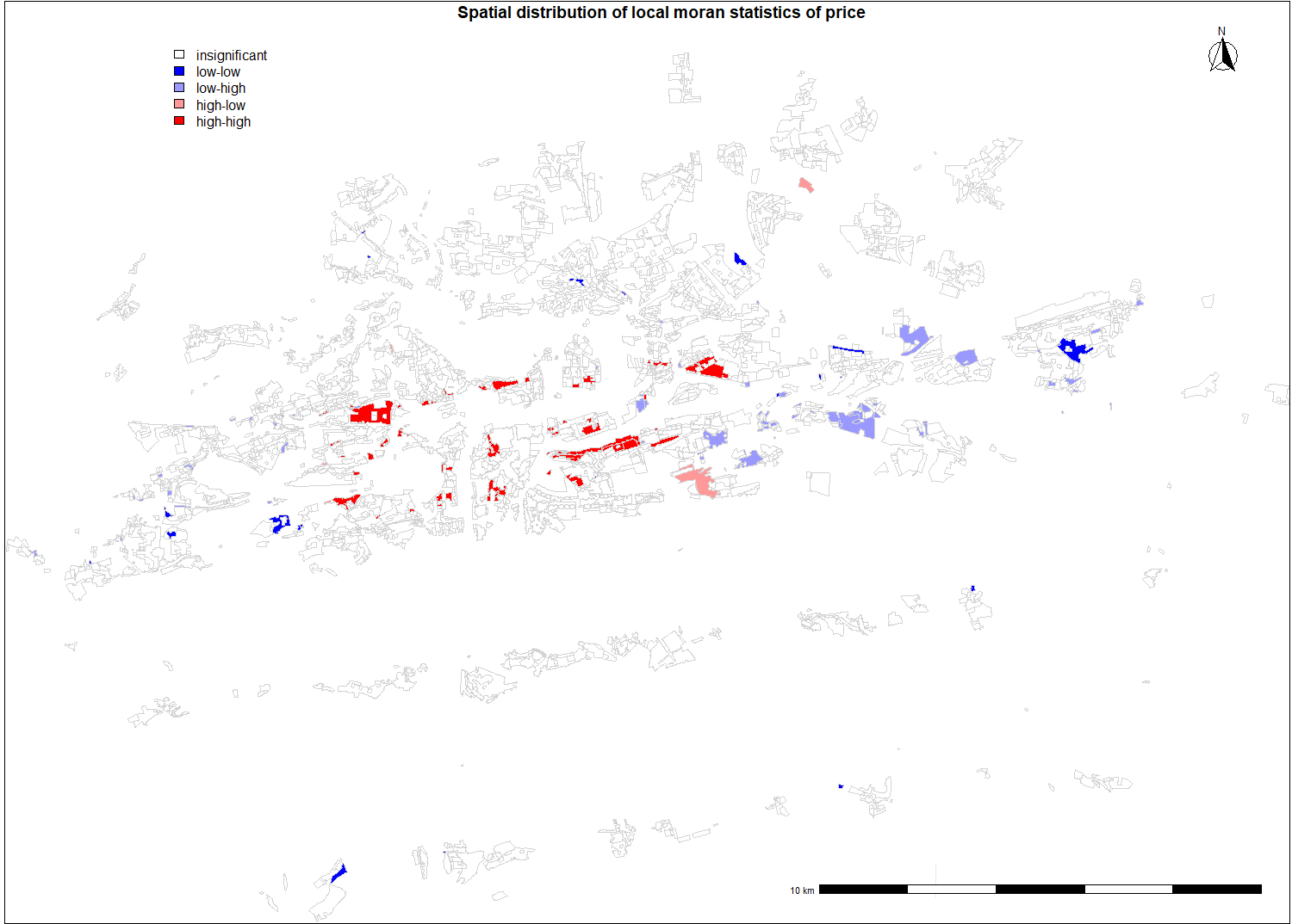
When investigating spatial distribution of local moran statistic of price, we can observe several high value polygons neighbouring with another high value polygons. The most apparent is red area north west. This neighborhood is called Hanspaulka and it consists of historical mansions. Smaller red polygons nearby consists of historical villas as well and they offer beautiful view on the Prague Castle which is nearby. The mentioned factors explain that these areas follow similar spatial clustering pattern. East of the Vltava river meander another large red polygon can be observed. This neighbourhood is called Harfa and it contains newly built luxury penthouses. Generally it can be concluded that high area regions neighbouring with another high area regions consist of either historical mansions, luxury penthouses or historical apartment blocks. Large blue polygons on the eastern part of the city contains mostly separated concrete panel apartment blocks, that were built during communist era. Although the outlying blue polygon on the south end of the city consist of detached houses, its located near highway and ring road crossing and no metro station is nearby, these factors contributes to result of low value of moran statistics.

Spatial distribution of moran statistics for price


Local Autocorrelation

Local spatial autocorrelation investigates the relationships between each observation and its surroundings, rather than providing a numerical summary of these relationships across space. Lets start by creating a moran plot for every variable. This type of graph depicts the spatial data against its spatially lagged values, augmented by reporting the summary of influence measures for the linear relationship between the data and the lag.

Moran plot for every variable is depicted on the figure ??. The plot is divided into four quadrants. In the upper right corner there is the first quadrant, upper left corner corresponds to the second, bottom left to the third and bottom right to fourth. For the Price variable (first plot), we can observe that the vast majority of the observations are clustered in the third quadrant. The third quadrant corresponds to low values surrounded by low values. The interpretation can be that the polygons with lower land price tends to be neighboured by another polygons with (relatively) low prices. In the empirical analysis chapter, when investigating spatial distribution of land price on the figure ??, similar cluster of low land price areas was identified North of the city center. We can see that in the second quadrant that corresponds to the low values surrounded by high values and in the fourth quadrant that corresponds to the high values surrounded by low values there is not many observations. It can be concluded that the city does not have many mixed neighbourhoods with respect to socioeconomic status of its inhabitants. Similar clustering pattern with most observations in the third quadrant can be observed for nearest bus stop distances. However this time the dispersion is more apparent. There is way more observations in the first quadrant, meaning that there are many polygons with relatively high distance to nearest bus station neighbouring with similar characteristic polygons. The observations for nearest metro,tram and train station distances seems to follow similar pattern as they are all aligned in diagonal line between first and third quadrants. This arrangement implies that there are either well connected neighbourhoods with low distances to nearest tram/train/metro stops or areas with bad connectivity and nothing between as there are only few points in the second and fourth quadrant.

Moran plots

How are particular moran statistics for each component distributed across spaced is analysed in dedicated chapters with links listed below:

Global Autocorrelation

To investigate whether the data does spatially cluster, the statistical model known as Moran’s Test is performed. The output of the model is Moran I test statistic, which is number between -1 and 1 where 1 determines perfect positive spatial autocorrelation (so the data are clustered), 0 implies that the data are randomly distributed and -1 corresponds to negative spatial autocorrelation, so dissimilar values tends to be next to each other. The table below shows Moran I test statistic and corresponding p value for each variable.


Variable

Moran I test statistic

p_value

Price

0.8429134579

<2.2e-16

Area

-0.0113012746

= 0.7068

Bus distance

0.5145050532

< 2.2e-16

Metro distance

0.8185449372

<2.2e-16

Train distance

0.8426067925

<2.2e-16

Tram distance

0.8311118133

< 2.2e-16

From the tests‘ outputs we can conclude that there is strong positive spatial autocorrelation for Price, Metro, Train and Tram distance variables and these data spatially cluster. Regarding the Area, the p value is above 0.05, so we can conclude that there is no significant spatial clustering of the data and as the test statistic is near zero, we can conclude that the data are most likely to be randomly distributed. For the Bus distance, the p value is below 0.05 so there is significant spatial pattern in the data however, as the test statistic is 0.514, the relationship is much weaker when comparing with other distance variables. It might suggests that there is some spatial pattern for local spots but not for the entire dataset.


Investigating Spatial Autocorrelation

In the empirical analysis it was concluded, that some variables tends to spatially cluster arround historical city center. To investigate, whether this clustering is statistically significant and how strong it is, spatial autocorrelation analysis is performed in this chapter.
Lets start with brief explanation of the spatial autocorrelation concept. Autocorrelation (whether spatial or not) is a measure of similarity (correlation) between nearby observations. A spatial autocorrelation measures how distance influences a particular variable. It quantifies the degree of which objects are similar to nearby objects. Variables are said to have a positive spatial autocorrelation when similar values tend to be nearer than dissimilar values. Spatial autocorrelation in a variable can be exogenous (it is caused by another spatially autocorrelated variable, e.g. rainfall) or endogenous (it is caused by the process at play, e.g. the spread of a disease) 1. There are two types of spatial autocorrelation – global and local. If the data are globally autocorrelated, the test statistics can tell us whether values in our map cluster together (or disperse) overall, but it won’t inform us about where specific clusters (or outliers) are. Local spatial autocorrelation investigates the relationships between each observation and its surroundings, rather than providing a numerical summary of these relationships across space. Both statistical models were applied and results were analysed in dedicated chapters.

Modelling

In this section, selected mathematical modelling methods will be applied to the processed data. First, inspection whether the data are spatially autocorrelated will be conducted. Afterwards, Geographically Weighted Regression will be applied, with Residential Land Price as dependent variable.

Nearest train station spatial distribution

The spatial distribution of the nearest train station distances for each polygon is depicted on the figure below. When inspecting the picture, it seems that the values are scattered as no low distances cluster of polygons is apparent and any other spatial pattern is not clear on the first look. When comparing with tram and metro spatial distribution of distances, we can observe that the areas on the eastern end of the city, near the border with Central Bohemian Region is better connected to the train network, rather than any other mode of public transport. This corresponds with the fact, that this part of the city has suburban character and it was designed for its residents to commute by rail.

Distance to nerest train station

Autorof thumbmail picture: Petr Novák:

Source


Data Analysis

In this section empirical data analysis will be conducted. Starting with the summary statistics of the dataset and then proceeding with spatial analysis of model’s variables. For each component of the model, dedicated section is listed below.

Calculating Distances

Using distance to nearest hub function in QGIS, for each public transport stop layer, the nearest hub distance to the centroid of each polygon is obtained. The snapshot from the nearest metro station distance output is plotted on the figure on the next page. The same procedure is applied to Tram,Train and Bus stops and by using spatial join, each hub distance is assigned to corresponding polygon. After converting the area of the polygons to square meters, all variables from the model scheme are obtained and the project will proceed with empirical data analysis.


Nearest bus stop spatial distribution

The spatial distribution of the nearest bus station distances for each polygon is depicted on the figure below. When comparing with tram and metro distances spatial distributions, the values for buses seems to be more randomly scattered, as there is no relatively low value cluster in the historical center or any apparent pattern, related with the distance to historical center. However, the comparison with previously inspected modes is not so accurate as the values‘ range is approximately eight times lower when comparing with tram and metro. It corresponds to the fact, that the bus network is way more densed as it can be observed on the figure.

Nearest bus stop spatial distribution

Nearest tram stop spatial distribution

Spatial distribution of the nearest tram distances is plotted below. When comparing with metro, similar pattern can be observed. However, more areas along the river seems to be better connected to the tram network. On the other hand, when inspecting the outskirts of the city, north-eastern part seems to be connected better to metro network. Compared with metro, the opposite can be observed on the western border of the city where the areas seems to be better connected to the tram network, as the distances are lower.

Nearest tram station distance spatial distribution