The best availability to the public transport system is in the city center. With increasing radius from the city center, the availability decreases as the highest values of the nearest public transport terminal distances tends to be clustered on the outskirts of the city, especially for all rail modes. It was found out that the municipalities that were joined to the capital most recently have smaller pubic transport service covarage and the activities in the development of the tram network was very small in the past decades. Furthermore, analysis, whether there are significant spatial clustering patterns was performed, by investigating Global and Local Autocorrelation in the data. For each explanatory variable and the dependent variable as well, neighbouring areas with similar spatial patterns were found.
The significant finding from this analysis is that the residential land price can be predicted using calculable distance variables. The distance from the centroid of the polygon to the nearest metro station is the strongest predictor. This finding confirms the role of the underground rail as core public transport system in Prague.
Měsíc: Září 2023
Analysing Spatial distributions of fitted model coefficients
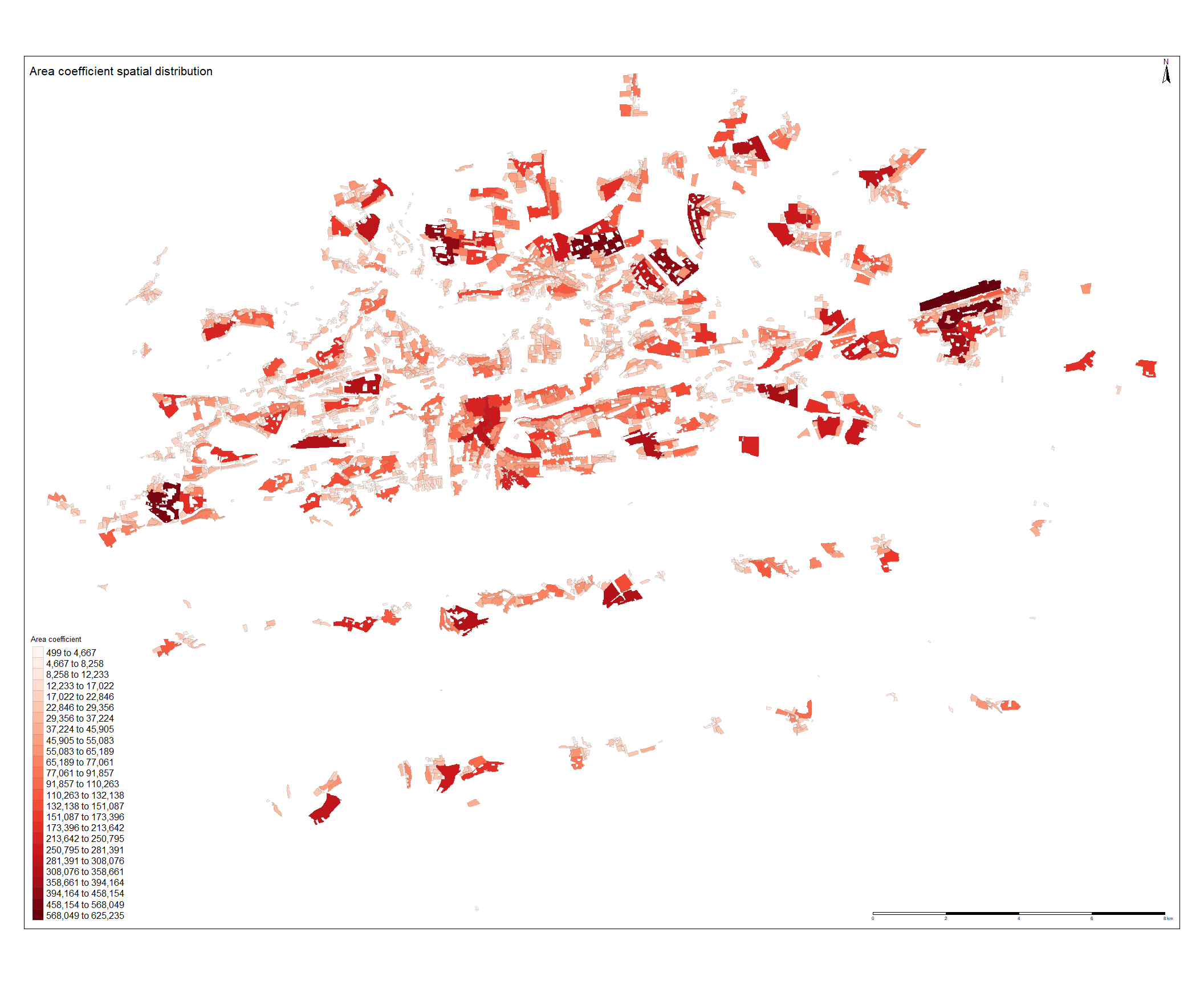
On the figure below, spatial distribution of the area coefficient estimate is ploted. The values seems to have plausible sign, indicating an increasing effect of the residential land price. Unlike for  , the highest values are not clustered in the historical city center. The highest values can be found on the eastern outskirt of the city, this is most likely to be caused by the actual polygon size as this one is the largest in the dataset. Another high values of the coefficients can be found north and west of the city center. The north area is called Troja and the west area is named Bertramka and these are the one of the most lucrative neighbourhood in the Prague consisting of luxurious mansions. The lowest values corresponds with the smallest polygons. Overall the values seems to be randomly scattered as no spatial clustering pattern is obvious.
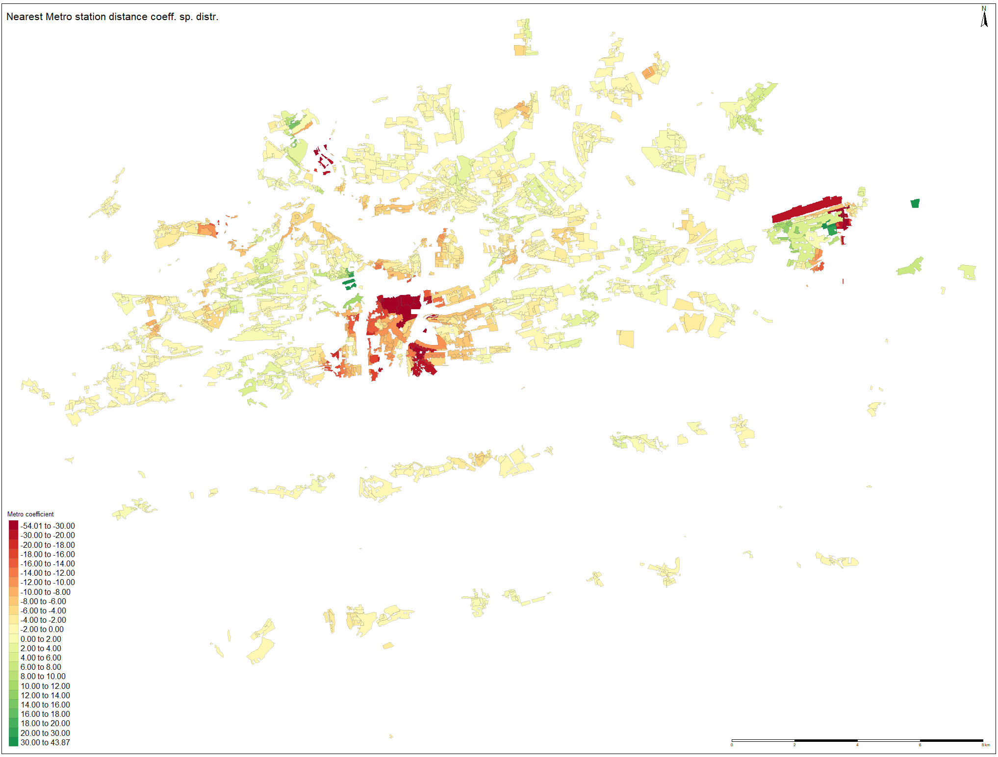
On the figures below, spatial distributions of the distance coefficients estimates are plotted. For the nearest metro distance coefficient, it can be observed that the lowest (red) values tends to be clustered in the city center. As the most valuable land is located there, it corresponds with the fact that the model assigns the strongest decreasing effect on these polygons. When going more from the center to outskirts it seems that the decreasing effect of metro distance on price tends to be weaker, as with increasing radius from city center, the polygons‘ color shade is getting lighter. Although some positively signed coefficients are present, especially in the Horní Počernice Municipality, their occurrence is not frequent. The green polygon near the city center is located very close to the Prague Castle and it is most likely affected by one of the highest price value.
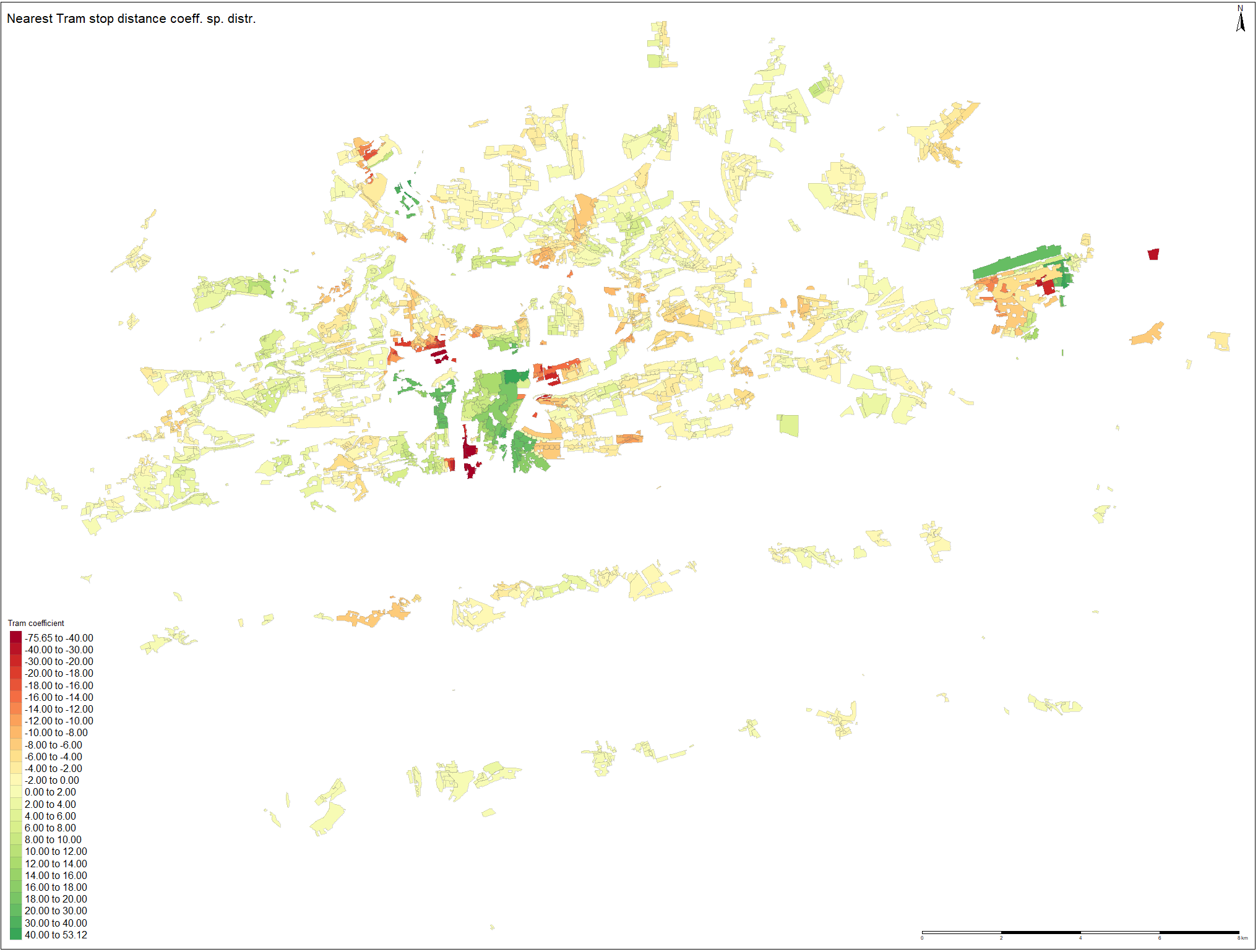
When investigating spatial distribution of the nearest tram stop distance coefficient, it can be observed that the model has assigned positively signed coefficients to the polygons in the city center. Although this not seem to be plausible result, it is most likely caused by the fact that the prices in the center are several times higher and it creates disbalances in the model. The solution can be to assign penalization for the most valuable residential land areas. However, this would have created bias in the model, violating linear relationship assumption between variables. Overall, the coefficients seems to have plausible sign on the eastern half of the city. On the western bank of the Vltava river and further, slightly positive values tends to cluster there. When comparing with metro coefficient estimates, the values for tram seems to be more randomly scattered as no buffering pattern is apparent in the distribution.
The Geographically weighted regression is a powerful tool to quantify how much the distance to nearest public transport terminal affects the residential land price. Although some limitations have appeared such as unplausible coefficients signs in some areas, in global average, the model presents plausible and realistic results.
When the multicolineratiy of the explanatory variables was found, several solutions were analyzed. By applying dimensionality reduction by Principal Component Analysis the explained variation in the data could have improved. However this solution was discarded as it would not be possible to correctly interpret, which public transport mode makes the largest contribution to the residential land price.
Fitting GWR model
After reprojecting the data to UTM grid, several types of Geographical Weighted Regression models were estimated. After fitting basic GWR model to the data, it has turned out that the suffers from multicolinearity of the independent variables. The coefficeints for distances in the full GWR model did not have plausible signs. It was expected for the coefficients to be negative which would imply that with increasing distance to nearest public transport terminal price of the land decreases. However, in some cases, these coefficients had positive sign, resulting in non realistic behaviour, compared with empirical findings. As the independent variables are highly correlated, Geographically Weighted Ridge and Geographically Weighted Lasso regression models were fitted, as in these models, the assumption of non-correlated independent variables is relaxed. Although these models provided improvement, some coefficients did not have plausible sign anyway. Therefore, reduction of the model was performed. The selection of the best performing model was based on the highest R^2 and the lowest AIC criterion. Several combination of the independent variables and kernel functions were investigated. Removing the nearest train and the nearest bus stop distance independent variables provided the best fit, in terms of the above mentioned criteria. The summary table of the model’s output from R is printed below.
Coefficient values imply that there is increasing effect of the area and decreasing effects of distances on price. In average, if the area increase by one square meter, the mean residential land price per square meter increase by 0.00763. In average, if the distance to nearest metro station increase by one meter, the mean price per square meter in Czech Crowns decrease by 0.624. If the distance to nearest tram stop increase by one meter, the mean price decrease by 0.183. GWR model provides a powerful predictor of the residential land price, explaining on average 84% of the variability in the dataset.
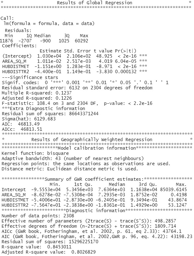
To investigate how the values of the coefficients are distributed across space, values of  estimates and the local values were mapped to corresponding polygons. The results are depicted on the next page. When investigating Local statistics we can observe that them model fits to the data very well in the city center, as the highest values of local can be found there. The lowest values of can be found south of the the city center, another low polygons can be found on the eastern band of the Vltava river meander. As the range of the magnitude is from 0.064 to 0.981 , it can be concluded that in the lightly shaded polygons the price of the residential land does not follow linear trend, based on the summary statistics of printed in the table ?? below, it can be concluded that these regions are minor and their effect on the model is low.
| Min. | 1st Qu. | Median | Mean | 3rd Qu | Max. |
|---|---|---|---|---|---|
| 0.06372 | 0.53994 | 0.70968 | 0.67972 | 0.83877 | 0.98145 |
Fitting Ordinary Least Squares Model
At first, an OLS model is investigated, summary output table is printed below:
| Estimate | Std. Error | t value | Pr(> |t|) | |
|---|---|---|---|---|
| (Intercept) | 10739.3519 | 323.2812 | 33.22 | 0.0000 |
| AREA_SQ_M | 0.0102 | 0.0025 | 4.04 | 0.0001 |
| HUBDISTBUS | -1.5666 | 0.9151 | -1.71 | 0.0870 |
| HUBDISTMET | -1.1445 | 0.1295 | -8.84 | 0.0000 |
| HUBDISTTRA | -0.0738 | 0.1357 | -0.54 | 0.5867 |
| HUBDISTTRAM | -0.4352 | 0.1164 | -3.74 | 0.0002 |
| Scores | F:65.78 (5,2302) | M. R^2: 0.125 | Adj. R^2: 0.1231 | AIC: 46814.1 |
With p value above 0.05, it can be concluded that bus and tram distance are not significant. This is most likely to be caused by multicolinearity of independent variables as all predictors are related with distance and even have the same unit. A model reduction is performed to have only significant variables. Summary table of the reduced model is printed below:
| Estimate | Std. Error | t value | Pr(>|t|) | |
|---|---|---|---|---|
| (Intercept) | 10304.5593 | 210.6201 | 48.92 | 0.0000 |
| AREA_SQ_M | 0.0101 | 0.0025 | 4.02 | 0.0001 |
| HUBDISTMET | -1.1507 | 0.1283 | -8.97 | 0.0000 |
| HUBDISTTRAM | -0.4400 | 0.1149 | -3.83 | 0.0001 |
| Scores | F:108.4 (3,2302) | M. R^2: 0.1237 | Adj. R^2: 0.1226 | AIC: 46813.49 |
Adjusted R squared metrics of the reduced model is 0.1226. It can be concluded that 12.26 percent of the variance in the data can be explained. Although model reduction was performed and model performance has slightly increased the model still fits poorly to the data.
Geographically Weighted Regression
Geographically weighted regression is a multivariate model that is taking into account non-stationarity across space. As the coefficients in GWR may vary across the inspected area, the method is an adequate tool to analyse local properties of the dependent variable.
Comparing with Ordinary least square regression, that generates a single equation for the global model:
(1) 
GWR constructs a separate equation for every feature in the dataset incorporating the dependent and explanatory variables of features falling within the bandwidth of each target feature. The Geographically weighted regression equation is
(2) 
where (ui, vi) represents the coordinates of the ith point in space. The cordinates for this model are the latitude and longitude coordinates of each polygons‘ centroid. The weight assigned is based on a distance decay function centered at location i and observations nearer to i are given greater weight than observations further away. The (global) ordinary least squares linear regression model assumes that the observations being
used are independent. As it was already explored in the previous chapter, this assumption is violated as there are significant spatial clustering patterns in the data. In Geographically Weighted Regression, this assumption is relaxed, as it allows for spatially varying coefficients by producing estimates
of the parameter at each data location, factoring in spatial heterogeneity.
Using OLS, the parameters for a linear regression model can be obtained by solving:
(3) 
The parameter estimates for GWR may be solved using a weighting scheme:
(4) 
The weights are chosen such that those observations near the point in space where the parameter estimates are desired to have more influence on the result than observations further away.
The Gaussian function is used for the weight calculation, the weight for the ith observation is:
(5) 
where  is the Euclidean distance between the location of observation i and location (u,v), and h is a bandwidth.
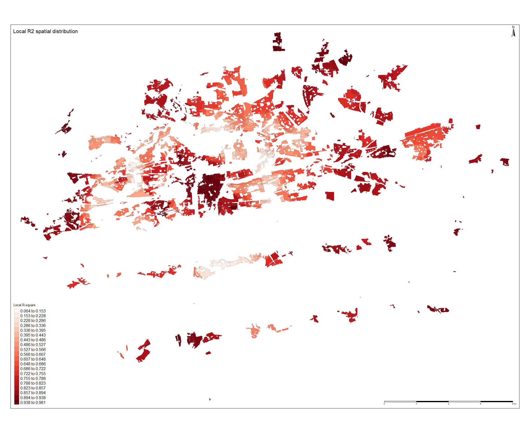
Spatial distribution of moran statistics for nearest train station distance
Spatial distribution of local Moran statistics for nearest train station distance is illustrated. It can be seen that the train network in Prague is shaped into a star with the main terminal (Praha Hlavní nádraží) in the city center. This corresponds with the original purpose of the system as it was designed to be used as a commuter rail for the suburban regions. There are 10 sections of the train lines that leads to Central Bohemian Region and the majority of low distance regions are aligned around them. Red polygons can be seen in the geographical center of the map however this cluster is completely surrounded by rail lines and it is well connected to other modes. North of the city center, large cluster of red polygons can be observed near Bohnice Municipality. It seems that this clustering pattern is repeating as some of these clustered areas has turned out red for buses and metro distances as well, implying poor connectivity which apparently leads to lower residential land prices in this region, concluding similar results with the findings in empirical analysis.
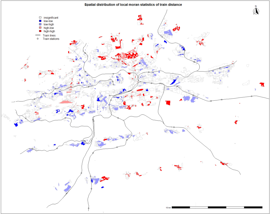
Spatial distribution of moran statistics for nearest tram stop distance
From visual inspection of the spatial distribution for nearest tram stop distance, it seems that the majority of the residential land areas is well connected to the tram network as these polygons tends to have short distance and they are neighboured by polygons with same characteristics in terms of tram network’s connectivity. Polygons with higher values of Moran statistics tends to be arranged in the north and east outskirts of the city. It can be seen from the figure that tram lines are missing in these neighbourhoods and their inhabitants have to rely on buses and individual forms of transportation. As mentioned before, these areas had been connected during the city expansion in 1922 or later, however it seems that no progress of expanding the tram network north east from center has been achieved since then. The situation will most likely remain same as no solution has been proposed yet and these areas aren’t included in the Official Development brochure for the next decade 1.
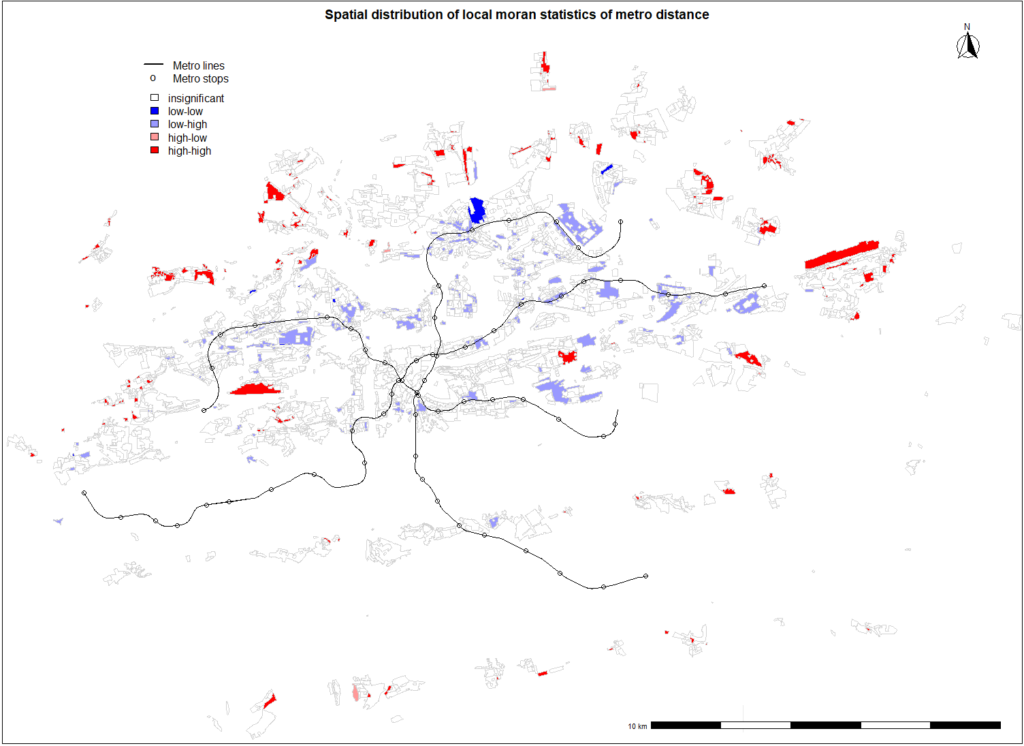
Spatial distribution of moran statistics for nearest metro station distance
When comparing spatial distribution of local moran statistics for metro with the same statistical model for bus, different spatial variation of Moran’s values can be observed. From all statistically significant polygons, the most frequent areas are light blue, corresponding to low values areas neighbouring with those with high value of Moran statistics. As all light blue areas are aligned near metro lines, this pattern confirms empirical observations. Besides one red polygon west of the city center, any other disconnected area lies on the outskirts of the city, where metro network doesn’t reach these neighbourhood. As the city will most likely expand, this can be early indicator of necessity to build ring line in the underground transportation system.
Spatial distribution of moran statistics for nearest bus stop distance
Spatial distribution of moran statistics for nearest bus stop distance is depicted. Note: The bus lines and stops are not plotted unlike for other modes. As the bus network and its stops are very densed, whole figure would become disorganized. We can observe that majority of statistical significant polygons are low values neighbouring with another low values. The implication from the model can be that these locations are well connected to the bus network. On the eastern end of the city we can observe a large red polygon. It is located in the Horní Počernice municipality, which is one of the most recent that was connected to Prague in 1974. The municipality has suburban character and this polygon is actually surrounding very frequently used train station so the usage of buses or trams was not prioritized during the development. From the figure it can be inspected that many regions are well connected to the bus network, however they are neighboured by areas with higher distances to nearest bus station. It seems that this pattern copies the historical development as these areas are located near the original border before the city expansion in 1922 1.

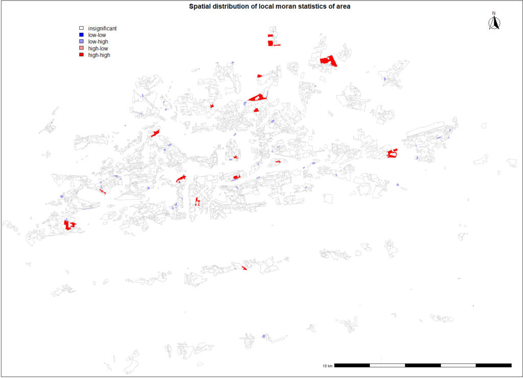
Spatial distribution of moran statistics for area
When investigating local clustering patterns of land area in square meters, large red polygons can be observed on the outskirt of the city. These neighbourhoods have suburban character consisting of detached houses with large gardens. Such characteristic is typical for larger areas that are neighbouring with another large areas. When interpreting small polygons in the city center, the only explanation with respect to area can be that these polygons consist of the most largest historical apartment blocks. As there are not many low value polygons neighbouring with another low value polygons, it can be concluded that the size of the residential areas is spatially dispersed which corresponds to the observations arrangement in the moran plot above.