Stating the assumptions of the general linear model:
- Normality of residuals
- Variance homogeneity
- Variance should be independent of location
- Linear relationship between x and y
By inspecting histograms we can conclude that we have broken the assumption of normality of residuals as the Ozone concentration does not seems to be normally distributed at all (it is most likely to be Poisson distributed or some derivative of Poisson distribution with similar shape, but for a general linear model, we assume it is normal). Also this problem can be potentially solved by applying logarithmic transformation.
By inspecting boxplots, we can conclude that the variance homogenity assumption is broken as the boxplots sizes are very disproportional when comparing to each other, that results in big differences in the interquartile ranges.
We start with a simple model without interactions and see which independent variables will be insignificant.
The model can be stated in the equation form as following:


Investigating Diagnostic Plots
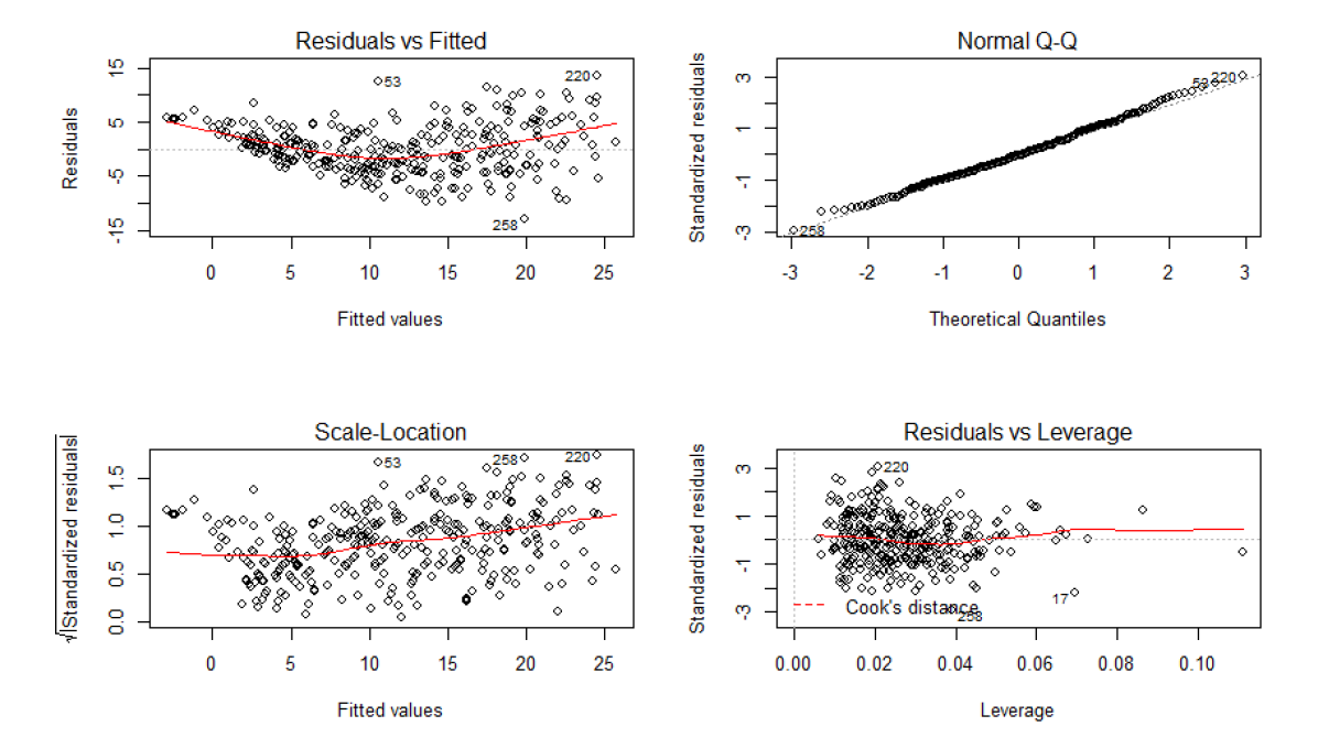
This model did not perform well in terms of significance of the independent variables (which was expected). The next options for general linear model might be to perform a transformation. Adding interactions and performing weighted analysis might be other options but we do not perform weighted analysis in this assignment to not loose the meteorological correctness of the model.