Poisson GLM
Compared with linear regression model, The Poisson log-linear model allows the variance to depend on the mean, and models the log of the mean as a linear function of the covariates.
Given a set of parameters θ and an input vector x, the mean of the predicted Poisson distribution, as stated above, is given by
![]()
Where ![]() is the vector of response variable,
is the vector of response variable, ![]() is vector of explanatory variables and
is vector of explanatory variables and ![]() is vector of parameters.
is vector of parameters.
By inspecting histogram of Ozone Concentration it seems that Poisson regression model can be good start as we can view the Ozone concentration as particles count and we use the log as the link function. We start without adding interactions or modifying the link function, we have 4 out of 8 variable significant on 5\% confidence level.
We can describe this model as follows:
![]()
Where ![]() is the i-th expected value of (E[
is the i-th expected value of (E[![]() ], which has to be positive,
], which has to be positive, ![]() is the intercept and
is the intercept and ![]() are the coefficients of predictors.
are the coefficients of predictors.
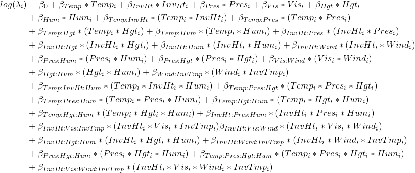
We try adding visibility and wind speed as factors, but we quickly figure out that it is not right to do so. Therefore, we start looking at interactions. We add all possible interactions, however, as discussed earlier, this is not a good approach, therefore, we start removing correlated variables as well as their interactions. We observe that even though the AIC scores don’t change much while we perform this tuning, the lowest AIC scores which we obtain are for the models when remove visibility (AIC = 1744.5) and when we remove the interactions between the heavily correlated variables (AIC = 1744.1). However, between these two models, the latter has quite a high number of statistically significant explanatory variables. We can also see this using the summary of the model (not presented here due to size issues but can be seen by running the code for fit3).
We performed tuning the Poisson regression model by backward selection from full model. When we removed right combination of parameters and interactions we got following model, where all parameters in the model are significant on 5 percent level, excluding the Temperature, which is significant on 10 percent. The best performing model in terms of significance of parameters and the lowest AIC for Poisson distribution is following:
