In the dataset there are 330 observations of the 9 variables. These data are for 330 days in 1976. All measurements are in the area of Upland, CA, east of Los Angeles. The dataset contains following columns:
- Ozone: Ozone concentration, ppm, at Sandbug AFB.
- Temp: Measured Temperature (degrees F)
- InvHt: Inversion base height (feet)
- Pres: Daggett pressure gradient (mm Hg)
- Vis: Visibily (miles)
- Hgt: Vandenburg 500 millibar height (m)
- Hum: Humidity (percent)
- InvTmp: Inversion base temperature (degrees F)
- Wind: Wind speed (mph)
We look at a summary of the dataset to look at the ranges of the various variables involved in the dataset. Then move to look at the structure of the dataset where it can be observed that Inverserion base temperature is the only float type variable in the dataset, all others are integers. The initial visualiziation in form of histograms, boxplots and cumulative densities is performed.
Boxplots and histogram analysis
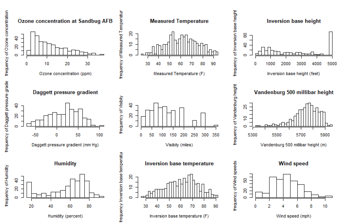
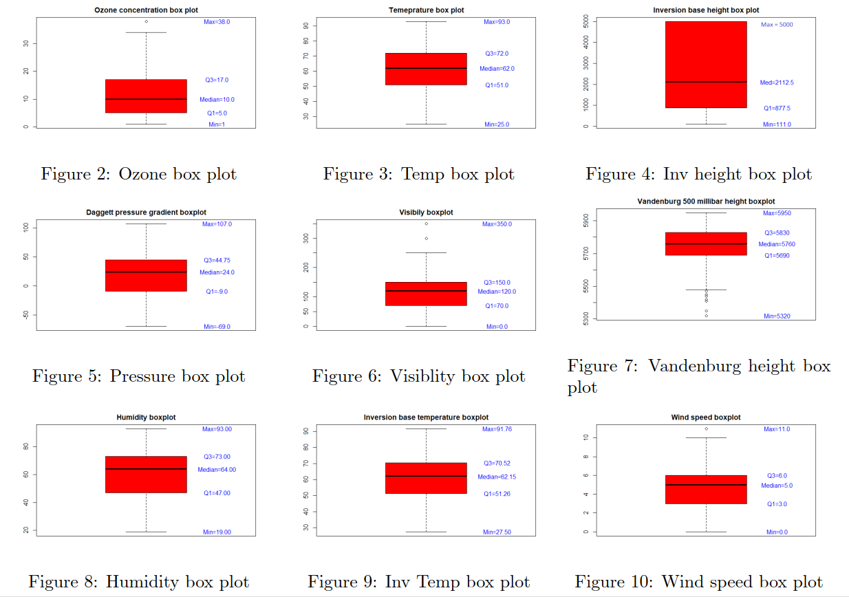
By observing the boxplots several conclusions can be stated: the ozone concentration tends to be skewed right. Some transformation might be necessary to improve model fit. Measured temperature seems to be normally distributed. In case of Inversion base height on the boxplot, we can see that distribution of observations is very disproportional. The most frequent value is 5000 feets with 95 observations, that is approximately 3 times more. This can be considered as a negatively skewed distribution. From statistical point of view, it would make sense to somehow handle the skewness, either by transforming the data or by assigning lower weight for the most frequent observations. However, from the empirical point of view we concluded to leave it because the skewness in the inversion base height in LA is most likely caused by the air pollution or anthroponic activities in general, as the city can be viewed as a heat island. When this effect is combined with the Santa Ana wind, it causes the inversion.
Regarding the visibility histogram, it seems to be slightly uniformly distributed, making groups of approximately 35 days, however it tends do decrease after the threshold of approx 200 miles. That makes sense in terms of that LA is located oceanic subtropical climate zone, where fogs are frequent.
Vandenburg 500 millibar height seems to be slightly negatively skewed but basically same implications as for the inversion base height can be stated, the more we will adjust data to get better fit, the less realistic the model will be from a meteorological point of view. The humidity seems to be multimodally distributed with first peak at 20 percent humidity that corresponds to winter period. The high humidities are most likely to occur during summer season, which is long in LA so the most of the observations fall into 6O to 80 percent.
The inversion base temperature seems to be normally distributed with slight negative skewness. The wind speeds may be slightly positively skewed but they are still centered around mean value which is 4.85 miles per hour.
Analysing correlation between variables
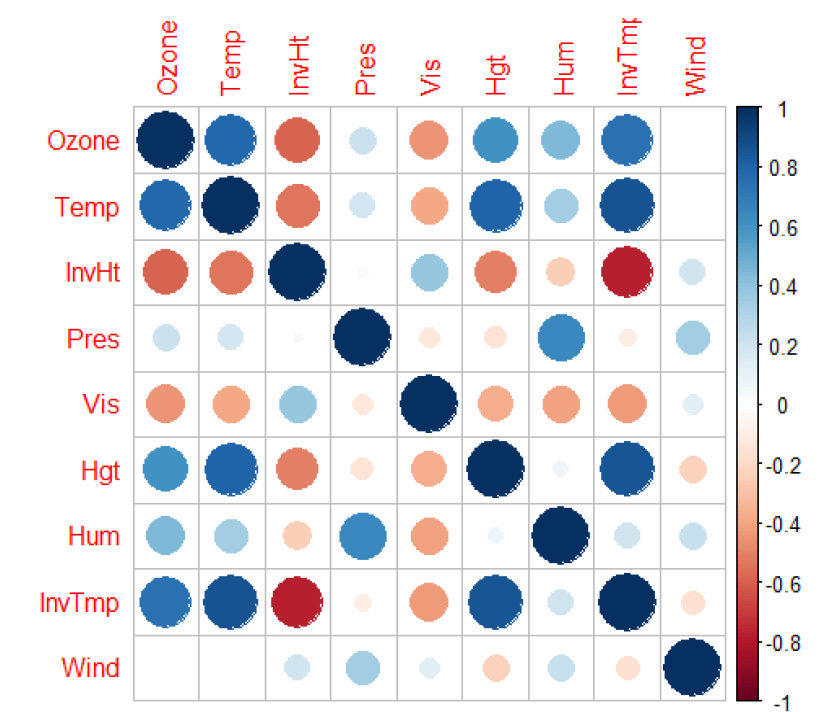
It can be observed that some variables are highly correlated. The strong correlation can be seen between Ozone and Temperature, Ozone and Inversion base temperature, Temperature and Vandenburg 500 millibar height. The strongest correlation can be found between Inversion base temperature and Measured temperature. Another strong correlation with negative sign can be seen between Inversion Height and Inversion base temperature. This will most likely cause some troubles especially in second questions as we broke assumption of general linear model.