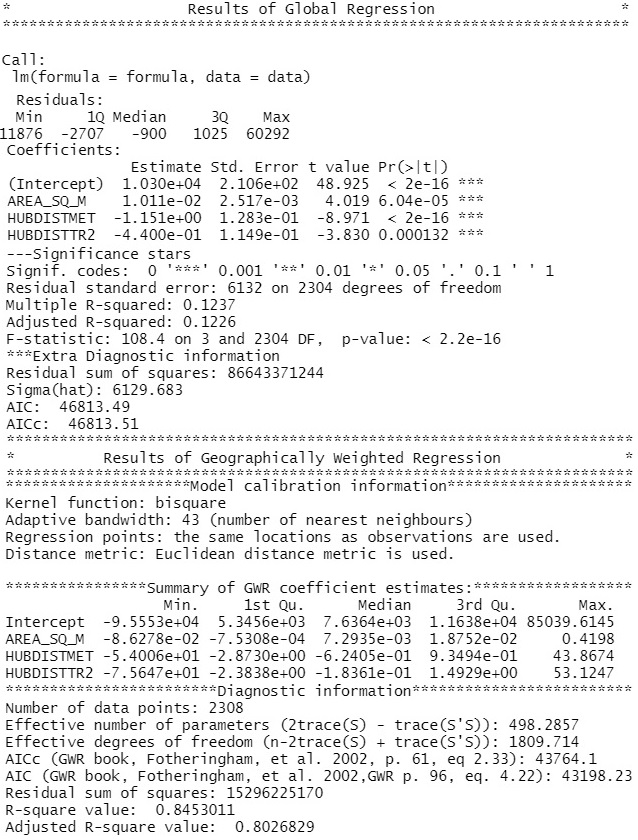
After reprojecting the data to UTM grid, several types of Geographical Weighted Regression models were estimated. After fitting basic GWR model to the data, it has turned out that the suffers from multicolinearity of the independent variables. The coefficeints for distances in the full GWR model did not have plausible signs. It was expected for the coefficients to be negative which would imply that with increasing distance to nearest public transport terminal price of the land decreases. However, in some cases, these coefficients had positive sign, resulting in non realistic behaviour, compared with empirical findings. As the independent variables are highly correlated, Geographically Weighted Ridge and Geographically Weighted Lasso regression models were fitted, as in these models, the assumption of non-correlated independent variables is relaxed. Although these models provided improvement, some coefficients did not have plausible sign anyway. Therefore, reduction of the model was performed. The selection of the best performing model was based on the highest R^2 and the lowest AIC criterion. Several combination of the independent variables and kernel functions were investigated. Removing the nearest train and the nearest bus stop distance independent variables provided the best fit, in terms of the above mentioned criteria. The summary table of the model’s output from R is printed below.
Coefficient values imply that there is increasing effect of the area and decreasing effects of distances on price. In average, if the area increase by one square meter, the mean residential land price per square meter increase by 0.00763. In average, if the distance to nearest metro station increase by one meter, the mean price per square meter in Czech Crowns decrease by 0.624. If the distance to nearest tram stop increase by one meter, the mean price decrease by 0.183. GWR model provides a powerful predictor of the residential land price, explaining on average 84% of the variability in the dataset.
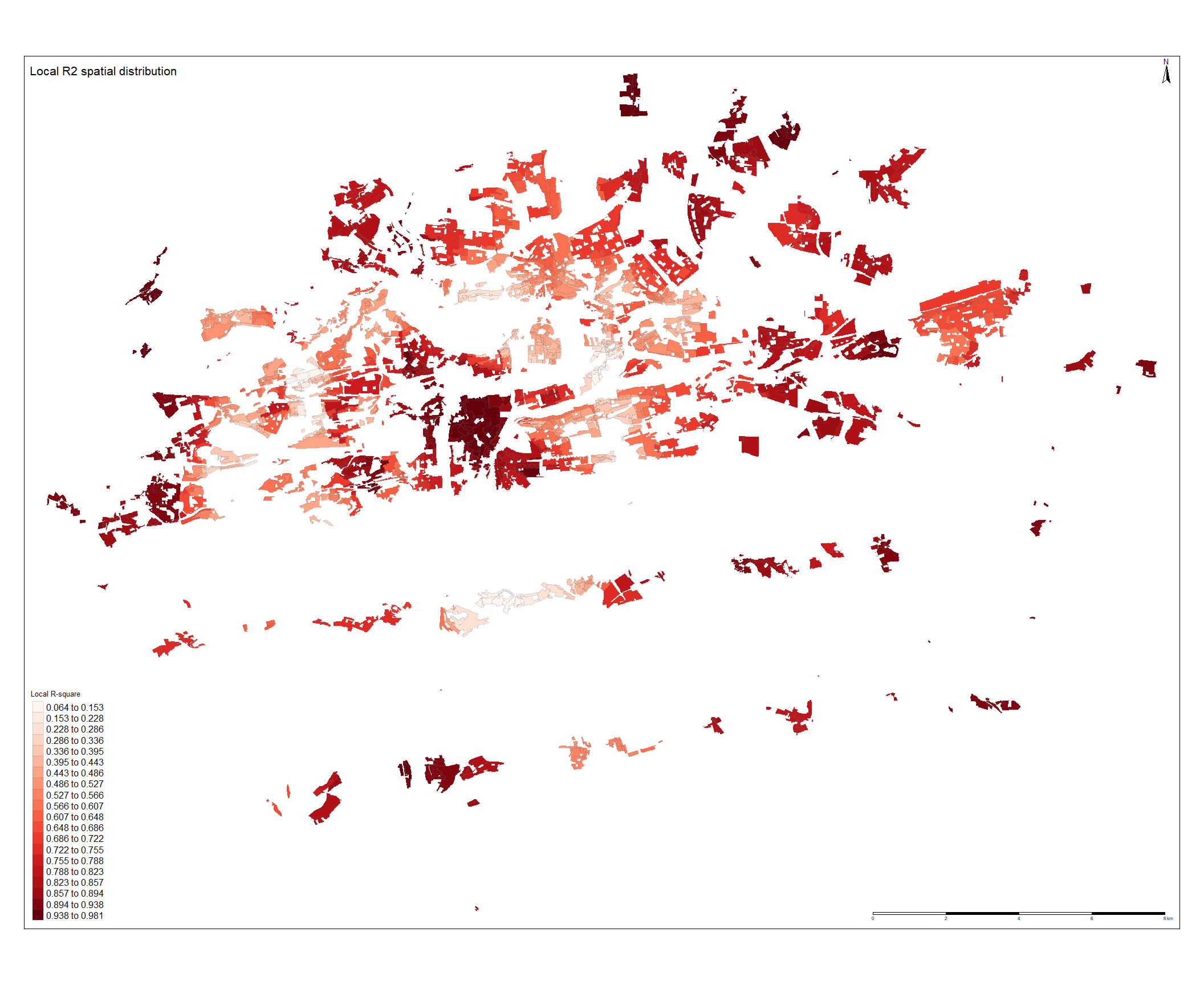
To investigate how the values of the coefficients are distributed across space, values of  estimates and the local
  values were mapped to corresponding polygons. The results are depicted on the next page. When investigating Local statistics we can observe that them model fits to the data very well in the city center, as the highest values of local can be found there. The lowest values of can be found south of the the city center, another low polygons can be found on the eastern band of the Vltava river meander. As the range of the magnitude is from 0.064 to 0.981 , it can be concluded that in the lightly shaded polygons the price of the residential land does not follow linear trend, based on the summary statistics of printed in the table ?? below, it can be concluded that these regions are minor and their effect on the model is low.
| Min. | 1st Qu. | Median | Mean | 3rd Qu | Max. |
|---|---|---|---|---|---|
| 0.06372 | 0.53994 | 0.70968 | 0.67972 | 0.83877 | 0.98145 |