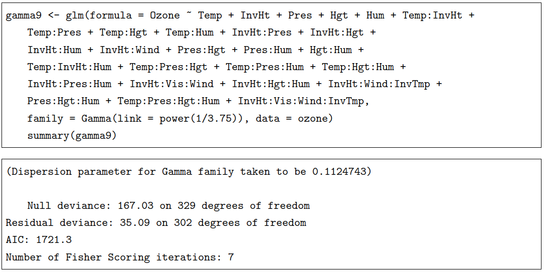
Although the coefficients seems to have very low value, which can be contraintuitive from the statistical point of view, from the empirical scope it makes perfectly sense. Our dependent variable is measured in parts per million. If we would have transformed the particles into length (or volume to be more cleared) unit scale, we would probably get them into micrometers or manometers scale compared with for example visibility, which is measured in miles.

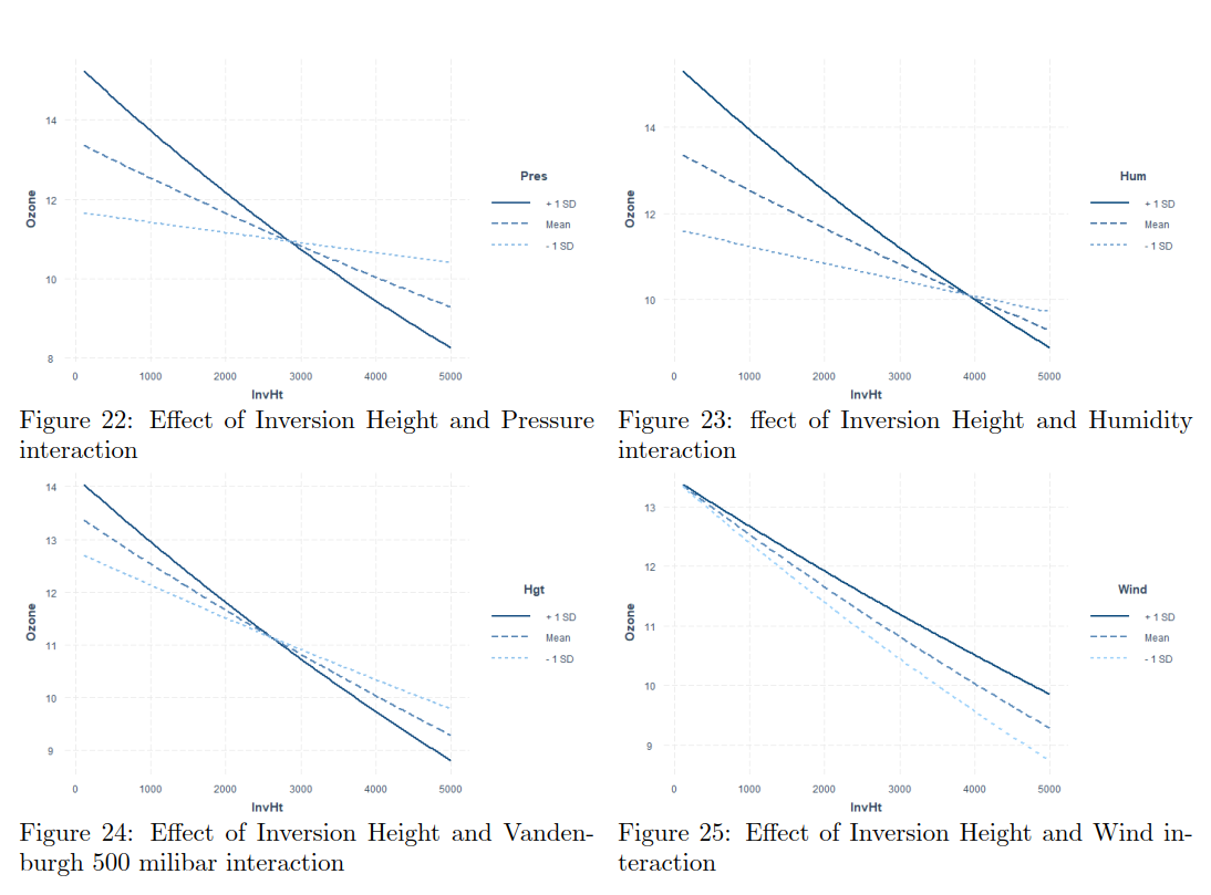
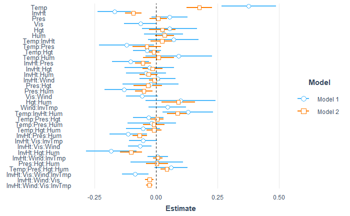
Considerieng sign of the coefficients, we can observe that additive effects without interactions (Temp, InvHt, Pres, Hgt, Hum) have all negative signs. We can see that the „strongest“ coefficient is for humidity, with value 1.091e+00. It would be easy to conclude that the humidity has the strongest effect on the ozone concentration, however particles modelling is very complex system that is very sensitive to disturbances of any kind. We can see that on modelled interactions. The coefficient with the lowest value of -2.037e-09 is for the interaction between Inversion base height, wind, visibility and Inversion base temperature, however it is still significant and we can conclude that even the tiniest increases or decreases in these variables can change the ozone concentration. The effect applies on any other interactions as well. We were surprised that in the final model, the wind speed is not significant. The intuition could deceive us that the ozone particles can be „blown away“ however it does not seems to be so easy. The wind speed seems to interacts with Inversion related variables (Inversion base height and Inversion Temperature, and also with Visibility) with more than 6 times lower values when comparing with Humidity. The weakness of the model also can be that it does not take into consideration directly effect of the air pollution. armful levels of ozone can be produced by the interaction of sunlight with certain chemicals emitted to the environment (e.g., automobile emissions and chemical emissions of industrial plants).
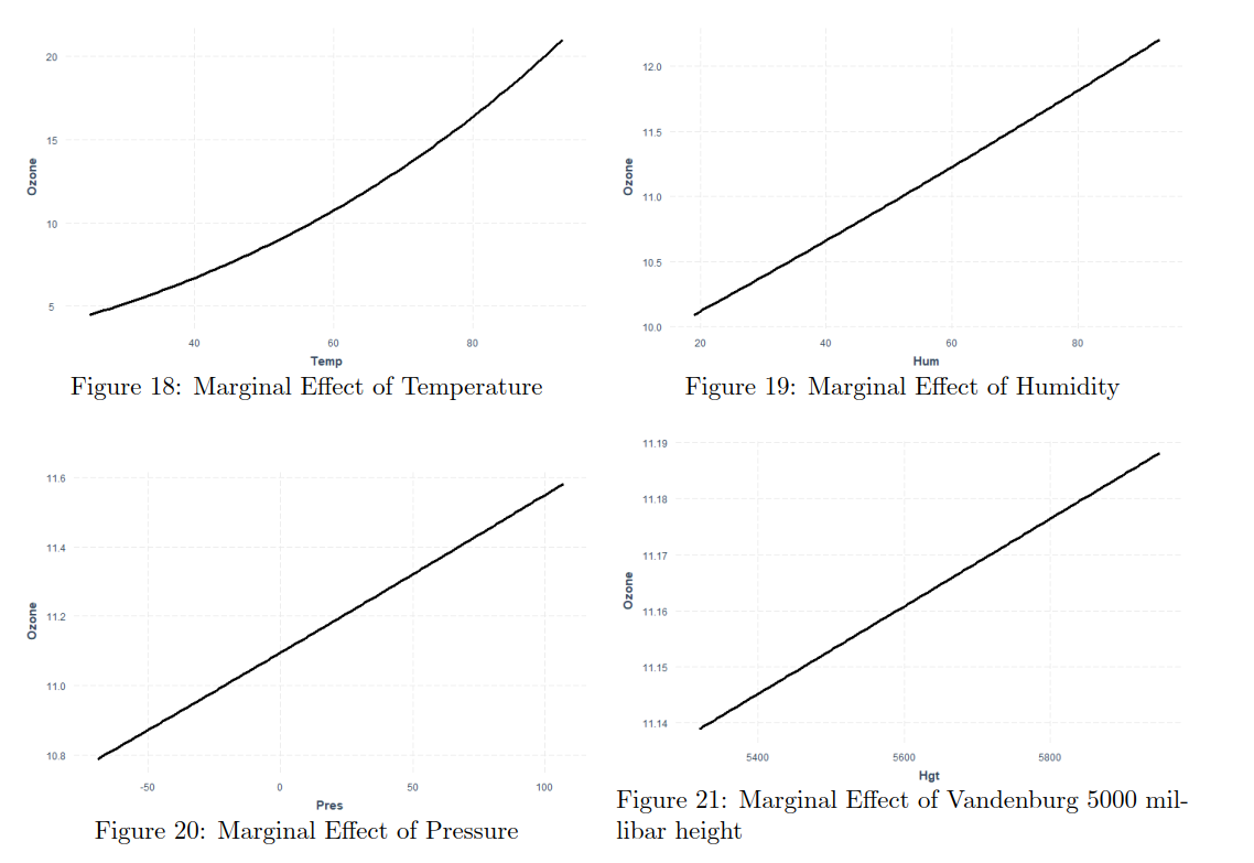
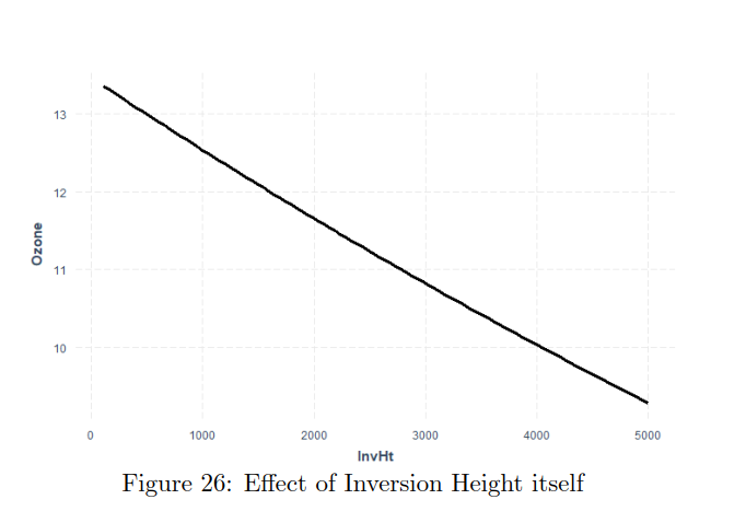
By plotting the additive effects we can observe that with Increasing Temperature, Pressure, Humidity, Vandenburg Height the ozone concentration increases. When increasing Inversion base Height Ozone concentration decreases. That makes perfect sense as An inversion traps air pollution, including ozone, close to the ground so low values of Inversion height mean that „clouds are up“ and when high then we have inversion. Therefore if we consider Inversion as the product of human activity, we can infer that air polluting increases the amount of harmful ozone particles in the air. Overall models seems to get plausible results (in terms of statistics), the weakness can be that the data are outdated (1976) and we have observations only from one measuring station, therefore we cannot infer impacts from other cities than Los Angeles.

When comparing the two approaches, the first thing that we need to note is that as we have already seen from the box plots which we have observed in data presentation, the assumption of constant variance which is required for classical GLM is violated. Therefore, using a classical GLM is not the right approach with this dataset. First a comparison was performed empirically as we know that we have several model assumptions broken in question 2. So we have concluded that there is no need to compare the classical glm with our final Generalized linear model by numerical measures.
Between the generalized linear models, we select the final Gamma model over the final Poisson model due to a better AIC score and also due to lower residual deviances. When comparing Poisson and Gamma model, we can see on the figure below(The Poisson model is represented by blue circles and Gamma by orange squares), that coefficients for both models have roughly same sign and therefore the effects of the explanatory variables will be in same „direction“ for both Poisson and Gamma model.

Gamma GLM

A random variable X that is gamma-distributed with shape k and scale θ is denoted by:

The Gamma distribution $Y \in G(\alpha,\beta x/\alpha$); Var[Y] = $(\beta x)^2)$
$$ \hat{\beta} = \frac{\alpha \sum y_i/x_i}{\sum alpha} = \frac{\sum \hat{\beta}_i}{k} $$
We try another generalized linear model using the Gamma family this time with the link function in this case being the inverse function. For this part, we look at two models: one containing all the interactions and one which is a minimal model just containing the explanatory variables.\\
In the first model, containing all the interactions, we see that a very decent fraction of the explanatory variables are statistically significant but the AIC score suffers a little compared to the Poisson model and it’s value is 1758.7 in this instance. In the minimal model, we get fewer statistically significant variables and the AIC score also takes a hit becoming 1848.6 now. Therefore, we can say that the model containing all the interactions performs better between the two but there might be scope for improvement using model reduction.\\
In addition to model reduction, there is another method to improve generalized linear models which is the use of different link functions. At first we used the inverse link function.
Afterwards we have found that cubic root link function is also suitable for gamma distributed models, thefore we specified the link function as „power (1/3)“ in R.

We found out that AIC scores improved (decreased) and also more variables were significant. We proceeded with tuning our link function and our model reduction to finally obtain a model with an AIC score as low as 1722 (referred to as gamma9 in our code) and all selected variables significant. This link function is defined as power (1/3.75).

Poisson GLM

Compared with linear regression model, The Poisson log-linear model allows the variance to depend on the mean, and models the log of the mean as a linear function of the covariates.

Given a set of parameters θ and an input vector x, the mean of the predicted Poisson distribution, as stated above, is given by

   

Where is the vector of response variable, is vector of explanatory variables and is vector of parameters.

By inspecting histogram of Ozone Concentration it seems that Poisson regression model can be good start as we can view the Ozone concentration as particles count and we use the log as the link function. We start without adding interactions or modifying the link function, we have 4 out of 8 variable significant on 5\% confidence level.
We can describe this model as follows:

   

Where is the i-th expected value of (E[], which has to be positive, is the intercept and are the coefficients of predictors.

We try adding visibility and wind speed as factors, but we quickly figure out that it is not right to do so. Therefore, we start looking at interactions. We add all possible interactions, however, as discussed earlier, this is not a good approach, therefore, we start removing correlated variables as well as their interactions. We observe that even though the AIC scores don’t change much while we perform this tuning, the lowest AIC scores which we obtain are for the models when remove visibility (AIC = 1744.5) and when we remove the interactions between the heavily correlated variables (AIC = 1744.1). However, between these two models, the latter has quite a high number of statistically significant explanatory variables. We can also see this using the summary of the model (not presented here due to size issues but can be seen by running the code for fit3).
We performed tuning the Poisson regression model by backward selection from full model. When we removed right combination of parameters and interactions we got following model, where all parameters in the model are significant on 5 percent level, excluding the Temperature, which is significant on 10 percent. The best performing model in terms of significance of parameters and the lowest AIC for Poisson distribution is following:

   

First of all let state the properties of generalized linear model:

• Exponential dispersion family
• Function of mean value linear
• Independent observations
• Variance function of mean

Compared with classical GLM, in the Generalized linear model, assumption of normally distributed observations with constant variance is relaxed. We look at two generalized linear models with different distributions of error terms – Poisson and Gamma.

 

 

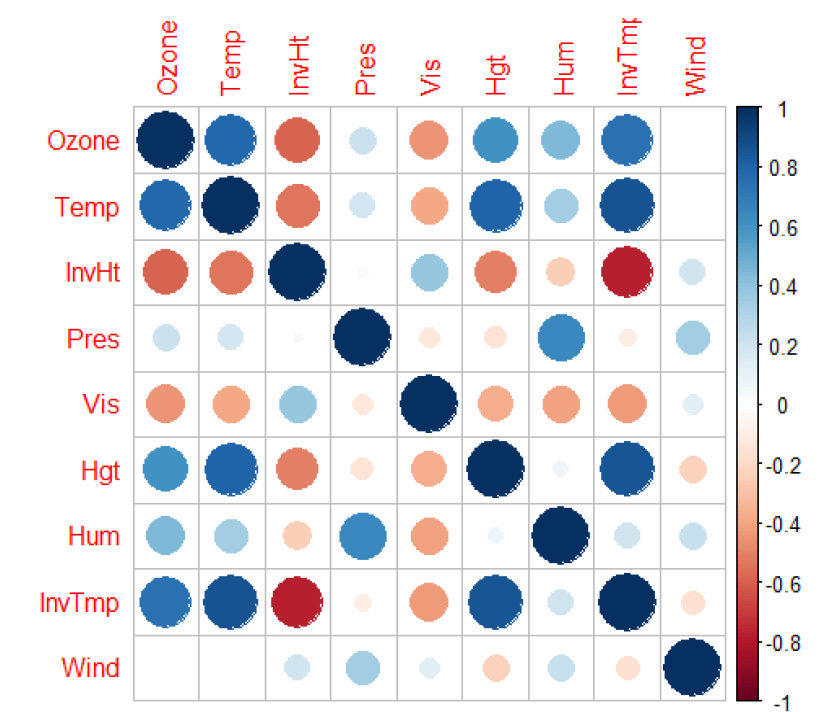
We start by looking at all the possible interactions between the explanatory variables, however, as we know from the theoretical aspect, we know that this approach will not work. The usual rule of thumb for adding interactions is to check the interactions between low correlated variables. When the and are uncorrelated, an interaction () might exist and impacts the correlation of the coefficients. As we have already seen, the explanatory variables have high correlations therefore the approach for checking the interactions between all the explanatory variables might not be a good approach.

Modelling using Step Function in R

Continuing the modelling using step function, which performs backward automatic model selection by comparing AIC. We will consider logarithmic and cubic root transformation of the dependent variable.

Cubic root transformed response variable

This model is stated in following equation:

   

Where is i-th fitted value, is the intercept and are parameters coefficients.

The model summary table is stated below. As you can see, several parameters are insignificant on 5 \% level, however step function still kept them in the model as removing them would have increased the amount of insignifant parameters and Adjusted R-squared value would have decreased.

Logarithmic transformed response variable

After discovering that cubic root transformation did not performed well in terms of significance of parameters, we decided to try logarithmic transformation of dependent variable ( The natural logarithm is being used). The model equation is stated below:

   

Where is i-th fitted value, is the intercept and are parameters coefficients.

Comparing two models

To choose which model performed better, we can calculate Akaike’s An Information Criterion for each model. The Akaike information criterion (AIC) is an estimator of prediction error and thereby relative quality of statistical models for a given set of data. Given a collection of models for the data, AIC estimates the quality of each model, relative to each of the other models. Thus, AIC provides a means for model selection. When comparing models fitted by maximum likelihood to the same data, the smaller the AIC the better the fit.

AIC of cubic root trasnformated model = 28.99864
AIC of log transformated model = 275.5243

By comapring AIC, we can conclude that cubic root transformed model provides better fit to the data.

Residual analysis

While inspecting Residuals vs Fitted plot, we can see that the observations are ordered in diagonal lines on the left half of the plot, that indicates some form of breaking of the model assumptions as the points should be randomly scattered, like starts on the night sky.

Regarding the Normal Q-Q plot, it is quite suprising that the most of the points lies on the diagonal line with only few outlying points on the tails. It can indicate overfitting as well however it is always quite tough to recognize optimal bias-variance tradeoff.

Scale-Location plot shows whether residuals are spread equally along the ranges of input variables (predictors). The assumption of equal variance (homoscedasticity) could also be checked with this plot. We can observe that majority of the points are located in the bottom half of the plot. The blue line is not much horizontal, these factors indicates breaking the assumption of variance homoscedasticity.

The Residuals vs. Leverage plots helps to identify influential data points on the model. The outliers can be influential and some points within a normal range in the model could be very influential. On the Residuals vs Leverage plot we can see one large cluster of points on the left half of the plot. Again the points should be scattered randomly to have the model assumption fullfilled.

The diagnostics plot help us to identify points that can be removed to potentially improve fit of the model. In our case, we could remove observation numbers 327, 196, 58 but we already know that we break model assumptions and the response variable does not seem to be normally distributed we decided not to spend more time into tuning of this model.

First, let’s try to transform Ozone concentration as hinted in the description and see if the model performance regarding to significance improves. We start by taking the square and the cube transform of the dependent variable but we see that on taking higher powers of the dependent variable, the adjusted R-squared value decreases from 0.557 to 0.4316 which signals that taking higher powers of the dependent variable might not be the right approach. A summary of these models along with some visual representation is present in the appendix.

We move on to working with the logarithmic and root transforms of the dependent variable. We see that on taking the log transform of the dependent variable, the adjusted R-squared increases to 0.695 and we observe that for this linear model, temperature and inversion height are significant explanatory variables.

We move to the square root transform of the dependent variable and see that the adjusted R-squared increases upto 0.7147 and inversion temperature joins the list of statistically significant explanatory variables. There are still numerous insignificant explanatory variables because of the high correlations that we had observed earlier but since the model seems to improving with decreasing function transformations on the dependent variable, we try the cube root and the fourth root transformations as well. We judge the performance of the model by improvements in the adjusted R-squared values and whether make explanatory variables become significant. We see that beyond the cube root of the dependent variable, we do not get any further improvements in the model, therefore we now start looking at interactions. The summary tables for all the models stated above as well as the summary plots can be found in the appendix.

Stating the assumptions of the general linear model:

• Normality of residuals
• Variance homogeneity
• Variance should be independent of location
• Linear relationship between x and y

By inspecting histograms we can conclude that we have broken the assumption of normality of residuals as the Ozone concentration does not seems to be normally distributed at all (it is most likely to be Poisson distributed or some derivative of Poisson distribution with similar shape, but for a general linear model, we assume it is normal). Also this problem can be potentially solved by applying logarithmic transformation.

By inspecting boxplots, we can conclude that the variance homogenity assumption is broken as the boxplots sizes are very disproportional when comparing to each other, that results in big differences in the interquartile ranges.

We start with a simple model without interactions and see which independent variables will be insignificant.
The model can be stated in the equation form as following:

   

Investigating Diagnostic Plots

This model did not perform well in terms of significance of the independent variables (which was expected). The next options for general linear model might be to perform a transformation. Adding interactions and performing weighted analysis might be other options but we do not perform weighted analysis in this assignment to not loose the meteorological correctness of the model.

In the dataset there are 330 observations of the 9 variables. These data are for 330 days in 1976. All measurements are in the area of Upland, CA, east of Los Angeles. The dataset contains following columns:

• Ozone: Ozone concentration, ppm, at Sandbug AFB.
• Temp: Measured Temperature (degrees F)
• InvHt: Inversion base height (feet)
• Pres: Daggett pressure gradient (mm Hg)
• Vis: Visibily (miles)
• Hgt: Vandenburg 500 millibar height (m)
• Hum: Humidity (percent)
• InvTmp: Inversion base temperature (degrees F)
• Wind: Wind speed (mph)

We look at a summary of the dataset to look at the ranges of the various variables involved in the dataset. Then move to look at the structure of the dataset where it can be observed that Inverserion base temperature is the only float type variable in the dataset, all others are integers. The initial visualiziation in form of histograms, boxplots and cumulative densities is performed.

Boxplots and histogram analysis

By observing the boxplots several conclusions can be stated: the ozone concentration tends to be skewed right. Some transformation might be necessary to improve model fit. Measured temperature seems to be normally distributed. In case of Inversion base height on the boxplot, we can see that distribution of observations is very disproportional. The most frequent value is 5000 feets with 95 observations, that is approximately 3 times more. This can be considered as a negatively skewed distribution. From statistical point of view, it would make sense to somehow handle the skewness, either by transforming the data or by assigning lower weight for the most frequent observations. However, from the empirical point of view we concluded to leave it because the skewness in the inversion base height in LA is most likely caused by the air pollution or anthroponic activities in general, as the city can be viewed as a heat island. When this effect is combined with the Santa Ana wind, it causes the inversion.

Regarding the visibility histogram, it seems to be slightly uniformly distributed, making groups of approximately 35 days, however it tends do decrease after the threshold of approx 200 miles. That makes sense in terms of that LA is located oceanic subtropical climate zone, where fogs are frequent.

Vandenburg 500 millibar height seems to be slightly negatively skewed but basically same implications as for the inversion base height can be stated, the more we will adjust data to get better fit, the less realistic the model will be from a meteorological point of view. The humidity seems to be multimodally distributed with first peak at 20 percent humidity that corresponds to winter period. The high humidities are most likely to occur during summer season, which is long in LA so the most of the observations fall into 6O to 80 percent.

The inversion base temperature seems to be normally distributed with slight negative skewness. The wind speeds may be slightly positively skewed but they are still centered around mean value which is 4.85 miles per hour.

Analysing correlation between variables

It can be observed that some variables are highly correlated. The strong correlation can be seen between Ozone and Temperature, Ozone and Inversion base temperature, Temperature and Vandenburg 500 millibar height. The strongest correlation can be found between Inversion base temperature and Measured temperature. Another strong correlation with negative sign can be seen between Inversion Height and Inversion base temperature. This will most likely cause some troubles especially in second questions as we broke assumption of general linear model.